
 Use the Index, Luke
 PostgreSQL Manual
Slides: juanignaciosl.github.io/sql-performance-explained/slides
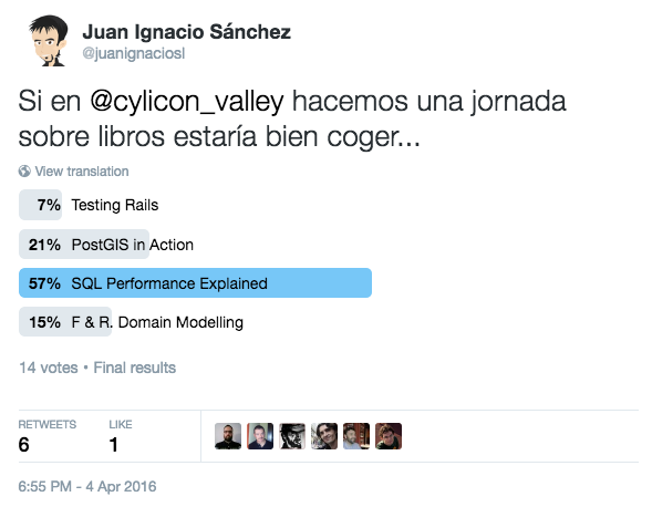
SQL Performance Explained
- Book and web
- Anatomy of an Index
- The Where Clause
- Performance and Scalability
- The Join Operation
- Clustering Data
- Sorting and grouping
- Partial results
- Modifying data
- Execution plans
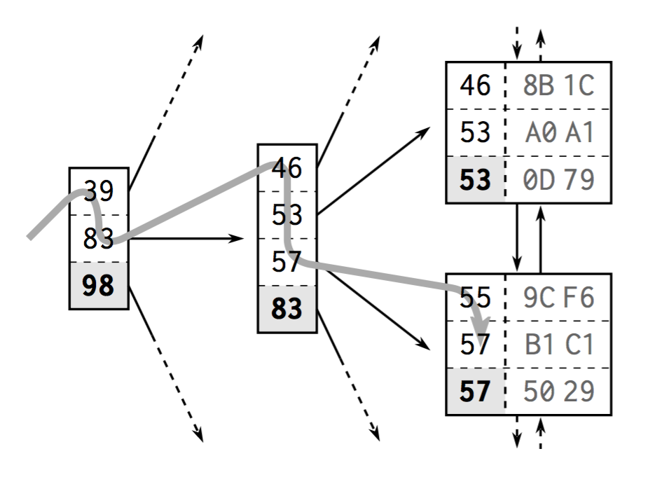
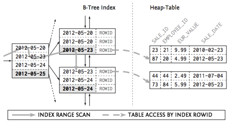
Anatomy of an Index
Anatomy of an Index
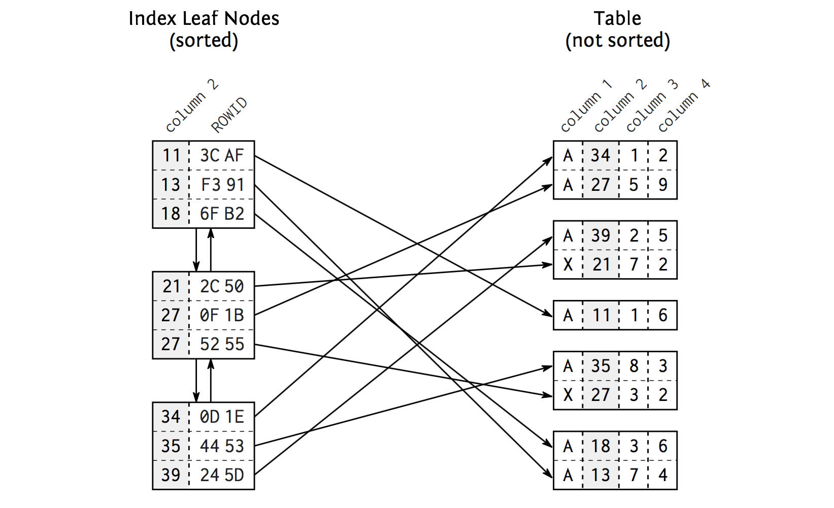
Anatomy of an Index
-
Index leaf nodes
- Doubly linked list
- (Doubly) Sorted: inside and among nodes
-
Database blocks
- Same size
- Unsorted and unlinked
Anatomy of an Index
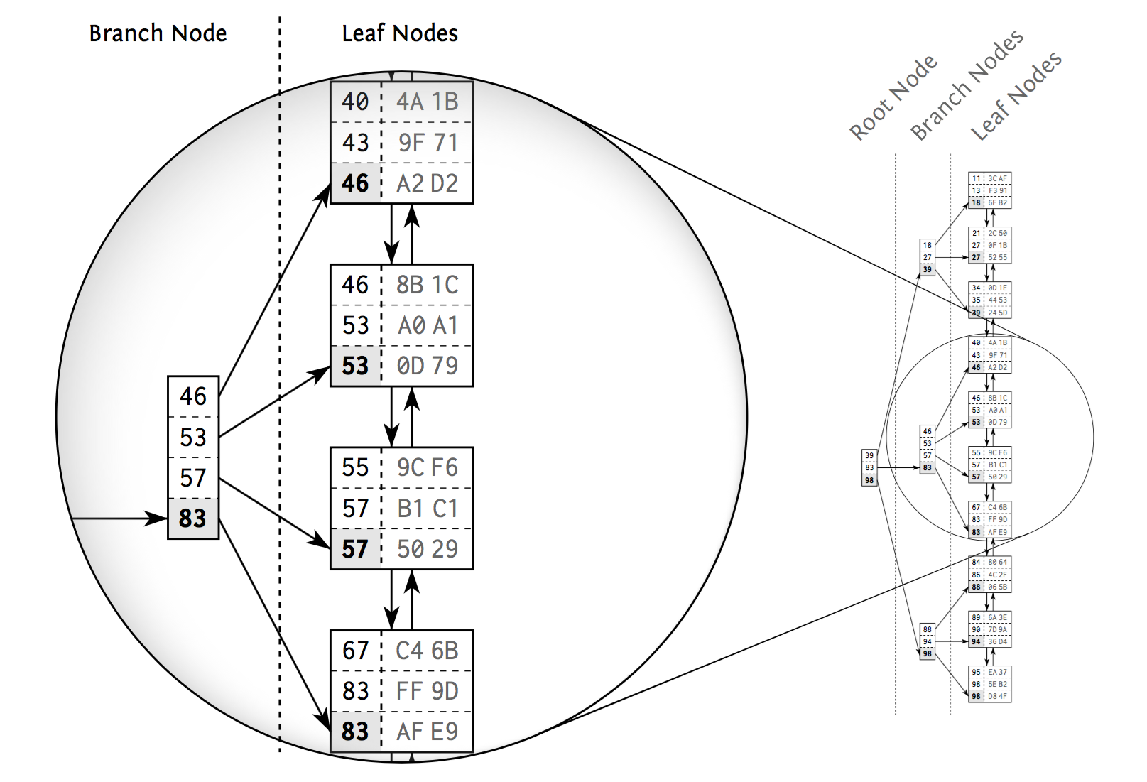
Anatomy of an Index
- Branch node entry -> biggest value
- Balanced search tree: tree depth equal at every position
- DB applies changes to the index and keeps the tree in balance
- ... thus causing maintenance overhead for write operations
Anatomy of an Index
Anatomy of an Index
The first power of indexing
- Tree balance allows accessing all elements with the same number of steps
- Logarithmic growth of the tree depth. Key tree depth factor: number of entries in each tree node. Databases often put hundreds.
B-Trees: slowness
-
Index lookup:
- tree traversal
- following the leaf node chain
- fetching the table data
- Database must read the next leaf node looking for more matching entries
- An index lookup needs to follow the leaf node chain
The Where Clause
The Where Clause
CREATE TABLE employees (
  employee_id integer not null PRIMARY key,
  subsidiary_id integer not null,
  first_name text,
  last_name text,
  date_of_birth DATE NOT NULL,
  phone_number character varying(1000) NOT NULL,
  enabled boolean default true
);

create unique index on employees (employee_id, subsidiary_id);

create index employees_last_name on employees(last_name);
The Where Clause
        Table "public.employees"
Column     |          Type           |  Modifiers
---------------+-------------------------+--------------
employee_id   | integer                 | not null
subsidiary_id | integer                 | not null
first_name    | text                    |
last_name     | text                    |
date_of_birth | date                    | not null
phone_number  | character varying(1000) | not null
enabled       | boolean                 | default true
Indexes:
"employees_pkey" PRIMARY KEY, btree (employee_id)
"enabled_employees" btree (last_name) WHERE enabled = true
"employees_last_name" btree (last_name)
Where clause: indexes - equality
explain analyze SELECT first_name, last_name
FROM employees WHERE employee_id = 123;
Where clause: indexes - equality
explain analyze SELECT first_name, last_name
FROM employees WHERE employee_id = 123;
Index Scan using employees_pkey on employees
    (cost=0.29..8.31 rows=1 width=16)
    (actual time=0.009..0.010 rows=1 loops=1)
Index Cond: (employee_id = 123)
Planning time: 0.310 ms
Execution time: 0.051 ms
Where clause: indexes - multiple columns
explain analyze SELECT first_name, last_name
FROM employees WHERE employee_id = 111
    and subsidiary_id = 333;
Where clause: indexes - multiple columns
explain analyze SELECT first_name, last_name
FROM employees WHERE employee_id = 111
    and subsidiary_id = 333;
Index Scan using employees_employee_id_subsidiary_id_idx
    on employees (cost=0.29..8.31 rows=1 width=16)
    (actual time=0.023..0.025 rows=1 loops=1)
Index Cond: ((employee_id = 111) AND (subsidiary_id = 333))
Planning time: 0.130 ms
Execution time: 0.056 ms
Where clause: indexes - multiple columns
explain analyze SELECT first_name, last_name
FROM employees WHERE subsidiary_id = 333;
Where clause: indexes - multiple columns
explain analyze SELECT first_name, last_name
FROM employees WHERE subsidiary_id = 333;
Index Scan using employees_employee_id_subsidiary_id_idx
    on employees (cost=0.29..1858.30 rows=1 width=16)
    (actual time=0.034..3.498 rows=1 loops=1)
  Index Cond: (subsidiary_id = 333)
Planning time: 0.101 ms
Execution time: 3.527 ms
A multicolumn B-tree index can be used with query conditions that involve any subset of the index's columns, but the index is most efficient when there are constraints on the leading (leftmost) columns.
PostgreSQL manual
Where clause: indexes - multiple columns
select * from employees where date_of_birth > TO_DATE($1, 'YYYY-MM-DD')
    and date_of_birth < TO_DATE($2, 'YYYY-MM-DD') and subsidiary_id = $3;
create index employees_date on
    employees(date_of_birth, subsidiary_id);
create index employees_date on
    employees(subsidiary_id, date_of_birth);
Where clause: indexes - multiple columns
Where clause: indexes - multiple columns
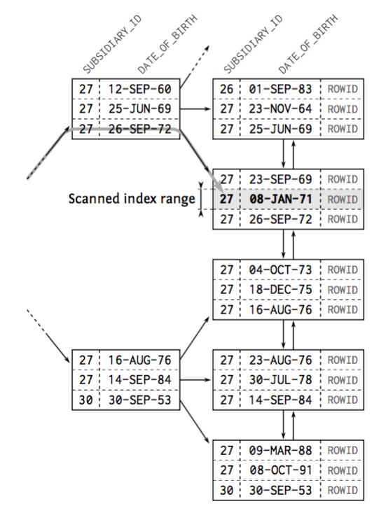
Where clause: indexes - multiple columns
Bitmap Heap Scan on employees
    (cost=14.54..22.28 rows=2 width=592) (actual time=0.069..0.071 rows=4 loops=1)
  Recheck Cond: ((date_of_birth > '1082-01-01'::date)
      AND (date_of_birth < '1083-01-01'::date) AND (subsidiary_id = 50))
  Heap Blocks: exact=3
  ->  Bitmap Index Scan on employees_date  (cost=0.00..14.54 rows=2 width=0)
      (actual time=0.064..0.064 rows=4 loops=1)
        Index Cond: ((date_of_birth > '1082-01-01'::date)
            AND (date_of_birth < '1083-01-01'::date) AND (subsidiary_id = 50))
Planning time: 0.365 ms
Execution time: 0.099 ms
Bitmap Heap Scan on employees
    (cost=4.34..19.58 rows=4 width=35) (actual time=0.045..0.051 rows=4 loops=1)
  Recheck Cond: ((subsidiary_id = 50) AND (date_of_birth > '1082-01-01'::date)
      AND (date_of_birth < '1083-01-01'::date))
  Heap Blocks: exact=3
  ->  Bitmap Index Scan on employees_date  (cost=0.00..4.34 rows=4 width=0)
      (actual time=0.037..0.037 rows=4 loops=1)
        Index Cond: ((subsidiary_id = 50) AND (date_of_birth > '1082-01-01'::date)
            AND (date_of_birth < '1083-01-01'::date))
Planning time: 0.481 ms
Execution time: 0.084 ms
The child plan node visits an index to find the locations of rows matching the index condition, and then the upper plan node actually fetches those rows from the table itself. Fetching rows separately is much more expensive than reading them sequentially, but because not all the pages of the table have to be visited, this is still cheaper than a sequential scan. PostgreSQL manual
Where clause: indexes - functions
explain analyze SELECT first_name, last_name
FROM employees WHERE last_name = 'LN 38'
Index Scan using employees_last_name on employees
    (cost=0.42..8.44 rows=1 width=16)
    (actual time=0.049..0.049 rows=1 loops=1)
  Index Cond: (last_name = 'LN 38'::text)
Planning time: 0.286 ms
Execution time: 0.082 ms
Where clause: indexes - functions
explain analyze SELECT first_name, last_name
FROM employees WHERE upper(last_name) = 'LN 38'
Seq Scan on employees
    (cost=0.00..2334.00 rows=500 width=16)
    (actual time=0.048..46.647 rows=1 loops=1)
Filter: (upper(last_name) = 'LN 38'::text)
Rows Removed by Filter: 99999
Planning time: 0.092 ms
Execution time: 46.672 ms
Where clause: indexes - functions
create index employees_upper_last_name
    on employees(upper(last_name));
Where clause: indexes - functions
explain analyze SELECT first_name, last_name
FROM employees WHERE upper(last_name) = 'LN 38'
Bitmap Heap Scan on employees
    (cost=12.29..775.05 rows=500 width=16)
    (actual time=0.070..0.070 rows=1 loops=1)
  Recheck Cond: (upper(last_name) = 'LN 38'::text)
  Heap Blocks: exact=1
  ->  Bitmap Index Scan on employees_upper_last_name
            (cost=0.00..12.17 rows=500 width=0)
            (actual time=0.065..0.065 rows=1 loops=1)
        Index Cond: (upper(last_name) = 'LN 38'::text)
Planning time: 0.360 ms
Execution time: 0.091 ms
Where clause: indexes - functions
explain analyze select * from employees where employee_id = 5;
explain analyze select * from employees where employee_id + 1 = 6;
Where clause: indexes - functions
explain analyze select * from employees where employee_id = 5;
Index Scan using employees_pkey on employees  (cost=0.29..8.31 rows=1 width=36) (actual time=0.014..0.015 rows=1 loops=1)
 Index Cond: (employee_id = 5)
Planning time: 0.075 ms
Execution time: 0.034 ms
explain analyze select * from employees where employee_id + 1 = 6;
Seq Scan on employees  (cost=0.00..2434.00 rows=500 width=36) (actual time=0.014..15.385 rows=1 loops=1)
 Filter: ((employee_id + 1) = 6)
 Rows Removed by Filter: 99999
Planning time: 0.066 ms
Execution time: 15.407 ms
Where clause: indexes - partial indexes
Partial indexes
create index enabled_employees on employees(last_name)
    where enabled = 't';
Where clause: indexes - parameterized queries
int subsidiary_id;
PreparedStatement command = connection.prepareStatement(
  "select first_name from employees where subsidiary_id = ?"
);
command.setInt(1, subsidiary_id);
- Prevents SQL injection
- Executing exactly same statement multiple times uses execution plan cache. The same SQL statement with different values is treated like different statements, recreating the execution plan.
Where clause: indexes - wrapping it up
- Master
explain plan - Avoid redundant indexes
- Avoid Seq Scan
- Keep an eye on queries and ORMs for function indexes
- ... since functions and transformations prevent index usage
- Index equality before ranges
- One multiple index is faster than two
- Parameterize as much as possible
- Disclaimer: actual results depend on data and filters
Performance and
Scalability
Performance and Scalability
The Join Operation
The Join Operation
- Normalized -> Denormalized
- 2 tables => 1 step (corollary: +2 tables => +1 step)
- Tables are pipelined, there's no intermediate materialization
- The more complicated the query, the harder the optimization, use bind variables!
- Three basic algorithms: nested loops, hash join and sort merge
The Join Operation: Nested Loops
- The right relation is scanned once for every row found in the left one
- Analogous to ORMs N+1 issue. Corollary: get to know your ORM and take control of joins
- Requires indexing of the join columns
The Join Operation: Nested Loops
- The right relation is scanned once for every row found in the left one
- Analogous to ORMs N+1 issue. Corollary: get to know your ORM and take control of joins
- Requires indexing of the join columns
- Good performance if the driving query returns a small result set
- Many B-tree traversals when executing the inner query
The Join Operation: Hash Join
- The right relation is first scanned and loaded into a hash table, using its join attributes as hash keys. Next the left relation is scanned and the appropriate values of every row found are used as hash keys to locate the matching rows in the table
- You can improve hash join performance by selecting fewer columns
- There is no need to index the join columns. Indexing independent where predicates improve performance
- Only one scan per table
- Symmetric
The Join Operation: Sort Merge
- Each relation is sorted on the join attributes before the join starts. Then the two relations are scanned in parallel, and matching rows are combined to form join rows
- Only one scan per table
The Join Operation: Sort Merge
- Each relation is sorted on the join attributes before the join starts. Then the two relations are scanned in parallel, and matching rows are combined to form join rows
- Only one scan per table
- Good for outer joins
- Good if input is sorted
Clustering Data
The Second Power of Indexing
Clustering Data: Index Filter Predicates
- Clustering data
- Store consecutively accessed data closely so thatit requires fewer IO operations
- You can only sort the physical table with one order...
- ... but you can create multiple indexes, with different orders
- Index filter predicates can be used not to improve range scan performance but to group consecutively accessed data together
Clustering Data: Index Filter Predicates
SELECT first_name, last_name, subsidiary_id, phone_number
FROM employees
WHERE subsidiary_id = ?
AND UPPER(last_name) LIKE '%INA%';
--------------------------------------------------------------
|Id | Operation | Name | Rows | Cost |
--------------------------------------------------------------
| 0 | SELECT STATEMENT | | 17 | 230 |
|*1 | TABLE ACCESS BY INDEX ROWID| EMPLOYEES | 17 | 230 |
|*2 | INDEX RANGE SCAN | EMPLOYEE_PK| 333 | 2 |
--------------------------------------------------------------
Predicate Information (identified by operation id):
---------------------------------------------------
     1 - filter(UPPER("LAST_NAME") LIKE '%INA%')
     2 - access("SUBSIDIARY_ID"=TO_NUMBER(:A))
Clustering Data: Index Filter Predicates
CREATE INDEX empsubupnam ON employees
    (subsidiary_id, UPPER(last_name));
Clustering Data: Index Filter Predicates
CREATE INDEX empsubupnam ON employees
    (subsidiary_id, UPPER(last_name));
--------------------------------------------------------------
|Id | Operation                   | Name       | Rows | Cost |
--------------------------------------------------------------
| 0 | SELECT STATEMENT            |            |   17 |   20 |
| 1 |  TABLE ACCESS BY INDEX ROWID| EMPLOYEES  |   17 |   20 |
|*2 |   INDEX RANGE SCAN          | EMPSUBUPNAM|   17 |    3 |
--------------------------------------------------------------
Predicate Information (identified by operation id):
---------------------------------------------------
   2 - access("SUBSIDIARY_ID"=TO_NUMBER(:A))
       filter(UPPER("LAST_NAME") LIKE '%INA%')
Clustering Data: Index-only scan
- Avoids accessing the table if the database has selected columns in the index itself
Clustering Data: Index-only scan
explain select subsidiary_id, last_name
    from employees where subsidiary_id < 5;
Bitmap Heap Scan on employees
    (cost=100.20..1089.58 rows=5150 width=12)
    (actual time=1.102..3.429 rows=5000 loops=1)
  Recheck Cond: (subsidiary_id < 5)
  Heap Blocks: exact=925
  ->  Bitmap Index Scan on employees_subsidiary_id_employee_id_idx
          (cost=0.00..98.92 rows=5150 width=0)
          (actual time=0.853..0.853 rows=5000 loops=1)
        Index Cond: (subsidiary_id < 5)
Planning time: 0.178 ms
Execution time: 3.867 ms
Clustering Data: Index-only scan
CREATE INDEX empsubupnam ON employees
    (subsidiary_id, last_name);
Clustering Data: Index-only scan
CREATE INDEX empsubupnam ON employees
    (subsidiary_id, last_name);
explain select subsidiary_id, last_name
    from employees where subsidiary_id < 5;
Index Only Scan using empsubupnam on employees
      (cost=0.42..170.54 rows=5150 width=12)
      (actual time=0.109..0.912 rows=5000 loops=1)
 Index Cond: (subsidiary_id < 5)
 Heap Fetches: 0
Planning time: 0.091 ms
Execution time: 1.244 ms
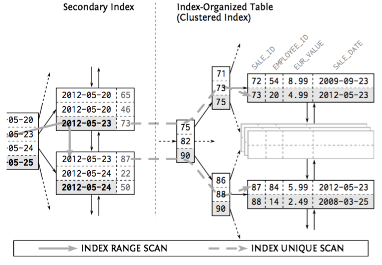
Clustering Data: Index-organized Tables
- Index-organized Tables (aka clustered index)
- Using an index as primary table store
- A B-tree index without a heap table
- Saves the space for the heap structure
- Every access on a clustered index is automatically an index-only scan
- Very inneficient on secondary indexes
Clustering Data: Index-organized Tables
Clustering Data: Index-organized Tables
Clustering data - wrapping it up
- Extend existing indexes to take advantage from filter predicates
- Extend existing indexes to take advantage from index-only scans
- Consider index-organized tables if you don't need more than one index
Sorting and grouping
Sorting and grouping
- Indexes provide ordered representations of the indexed data...
- ...so we can use indexes to avoid the sort operation to satisfy an order by clause
- Indexed order by execution also returns the first results without processing all input data, it's executed in a pipelined manner
Sorting and grouping
explain analyze select * from sales order by sale_date;
Sort  (cost=122200.04..124450.04 rows=900000 width=24)
    (actual time=810.872..1007.881 rows=900000 loops=1)
 Sort Key: sale_date
 Sort Method: external merge  Disk: 29912kB
 ->  Seq Scan on sales
    (cost=0.00..14733.00 rows=900000 width=24)
    (actual time=0.006..113.583 rows=900000 loops=1)
Planning time: 0.112 ms
Execution time: 1074.673 ms
Sorting and grouping
create index sales_date on sales(sale_date);
explain analyze select * from sales order by sale_date;
Sorting and grouping
create index sales_date on sales(sale_date);
explain analyze select * from sales order by sale_date;
Index Scan using sales_date on sales
    (cost=0.42..29120.43 rows=900000 width=24)
    (actual time=0.024..247.604 rows=900000 loops=1)
Planning time: 0.118 ms
Execution time: 315.568 ms
Sorting and grouping
- Execution time: 1074.673 ms -> 315.568 ms :-) (x0.3)
- Planning time: 0.112 ms -> 0.118 ms :-| (~=)
Sorting and grouping
- Execution time: 1074.673 ms -> 315.568 ms :-) (x0.3)
- Planning time: 0.112 ms -> 0.118 ms :-| (~=)
- cost=122200.04..124450.04 -> 0.42..29120.43 :-) (x0.2)
Sorting and grouping
- Execution time: 1074.673 ms -> 315.568 ms :-) (x0.3)
- Planning time: 0.112 ms -> 0.118 ms :-| (~=)
- cost=122200.04..124450.04 -> 0.42..29120.43 :-) (x0.2)
TL;DR: cost is not always an accurate measure
For a query that requires scanning a large fraction of the table, an explicit sort is likely to be faster than using an index because it requires less disk I/O due to following a sequential access pattern
Cost can increase because clustering factor of the new index is worse
[Clustering Factor]
[Clustering Factor]
- Performance benchmark
- Correlation between index order and table order
- Indirect measure of the probability that two succeeding index entries refer to the same table block
- Used by the optimizer to calculate the cost value of the TABLE ACCESS BY INDEX ROWID operation
- Good on chronological data, bad in random
- Indexes with good clustering factor don't benefit from performance advantage on index-only scan
[Clustering Factor]
select tablename, attname, correlation from pg_stats where
    schemaname = 'public';
 tablename |    attname    | correlation
-----------+---------------+-------------
 employees | date_of_birth |    0.976956
 employees | phone_number  |    0.801827
 employees | enabled       |    0.935313
 sales     | employee_id   |           1
 sales     | subsidiary_id |   0.0180426
 sales     | sale_id       |           1
 sales     | amount        |           1
 sales     | sale_date     |          -1
 employees | employee_id   |    0.976954
 employees | subsidiary_id |   -0.022466
 employees | first_name    |    0.801827
 employees | last_name     |    0.801827
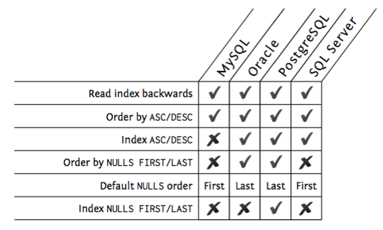
Sorting and grouping: asc/desc and nulls
- Databases can read indexes in both directions
Sorting and grouping: grouping
Algorithms- Temporary hash
- Sort/group
Sorting and grouping: grouping
Algorithms- Temporary hash
- Sort/group
- With already sorted indexes
Partial results
Partial results: retrieving top-n
- Fetch only the first rows of a query and then closing the statement
Partial results: retrieving top-n
- Fetch only the first rows of a query and then closing the statement - the optimizer cannot foresee that when preparing the execution plan
Partial results: retrieving top-n
- Fetch only the first rows of a query and then closing the statement - the optimizer cannot foresee that when preparing the execution plan
LIMIT { count | ALL }
OFFSET start
OFFSET start { ROW | ROWS }
FETCH { FIRST | NEXT } [ count ] { ROW | ROWS } ONLY
Partial results: paging - offset method
SELECT * FROM sales ORDER BY sale_date DESC OFFSET 10
FETCH NEXT 10 ROWS ONLY;
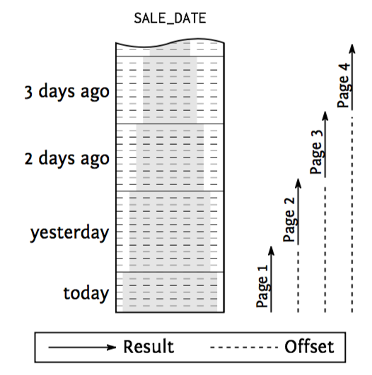
The offset method
Partial results: paging - seek method
SELECT * FROM sales WHERE sale_date < ?
ORDER BY sale_date DESC FETCH FIRST 10 ROWS ONLY;
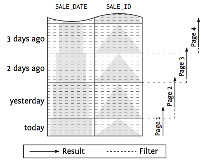
The seek method
Partial results: paging
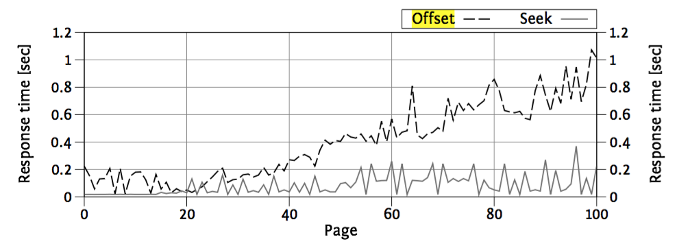
Offset vs seek performance
Partial results: paging
-
Offset method
- Simple and syntax support in SQL and ORMs
- Poor performance
- Pages drift on new items
-
Seek method
- More complicated
- Good performance
- Pages don't drift on new items
Modifying data
Modifying data: insert
The more indexes a table has, the slower the execution becomes.- Store the row in any block with free space
-
Update indexes
- Find the correct leaf node
- Split leaf node if it hasn't free space
Modifying data: insert
The more indexes a table has, the slower the execution becomes.- Store the row in any block with free space
-
Update indexes
- Find the correct leaf node
- Split leaf node if it hasn't free space
- Add the entry to each and every index
- Balance tree on split
Modifying data: delete
Similar to insert but, since it also searches, it takes advantage of indexes.- Find matches
- Delete the row
- Update indexes
Modifying data: delete
Similar to insert but, since it also searches, it takes advantage of indexes.- Find matches
- Delete the row
- Update indexes
- Takes advantage of indexes for search
- Removes the entry from each and every index
- Balance the tree on compacting
Modifying data: update
- Removes the old one and adds the new one
- Takes as much as delete + insert
- Sensitive to update only changes (ORMs!)
Execution plans
PostgreSQL
Execution plans
PREPARE stmt(int) AS SELECT $1;
Execution plans
PREPARE stmt(int) AS SELECT $1;
EXPLAIN EXECUTE stmt(1);
Execution plans
PREPARE stmt(int) AS SELECT $1;
EXPLAIN EXECUTE stmt(1);
Result (cost=0.00..0.01 rows=1 width=0)
- 0.00
- Startup cost
- 0.01
- Total cost for the execution if all rows are retrieved
Execution plans
PREPARE stmt(int) AS SELECT $1;
EXPLAIN EXECUTE stmt(1);
Result (cost=0.00..0.01 rows=1 width=0)
- 0.00
- Startup cost
- 0.01
- Total cost for the execution if all rows are retrieved
DEALLOCATE stmt;
Execution plans
EXPLAIN ANALYZE EXECUTE stmt(1);
EXPLAIN ANALYZE UPDATE EMPLOYEES
    SET LAST_NAME = 'x' WHERE EMPLOYEE_ID = 1;
Update on employees  (cost=0.29..8.31 rows=1 width=34)
    (actual time=0.261..0.261 rows=0 loops=1)
  ->  Index Scan using employees_pkey on employees
      (cost=0.29..8.31 rows=1 width=34)
      (actual time=0.136..0.138 rows=1 loops=1)
        Index Cond: (employee_id = 1)
Planning time: 0.095 ms
Execution time: 0.297 ms
Execution plans: index and table access
- Seq Scan
- Index Scan
- Index Only Scan
- Bitmap Index Scan / Bitmap Heap Scan / Recheck Cond
Execution plans: Join Operations
- Nested Loops
- Hash Join / Hash
- Merge Join
Execution plans: Sorting and Grouping
- Sort / Sort Key
- GroupAggregate
- HashAggregate
Execution plans: Top-N Queries
- Limit
- WindowAgg
Execution plans: Distinguishing Access and Filter-Predicates
- Access Predicate (“Index Cond”)
- Start and stop conditions of the leaf node traversal
- Index Filter Predicate (“Index Cond”)
- Applied during the leaf node traversal only. They do not contribute to the start and stop conditions and do not narrow the scanned range
- Table level filter predicate (“Filter”)
- Predicates on columns that are not part of the index are evaluated on the table level
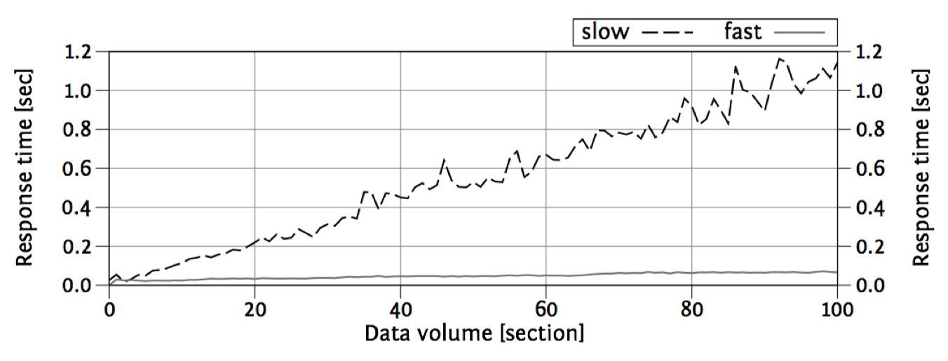
PostgreSQL execution plans do not show index access and filter predicates separately—both show up as “Index Cond”. That means the execution plan must be compared to the index definition to differentiate access predicates from index filter predicates.
Execution plans: Distinguishing Access and Filter-Predicates
CREATE TABLE scale_data (
     section NUMERIC NOT NULL,
     id1     NUMERIC NOT NULL,
     id2     NUMERIC NOT NULL
  );
CREATE INDEX scale_data_key ON scale_data(section, id1);
Execution plans: Distinguishing Access and Filter-Predicates
PREPARE stmt(int) AS SELECT count(*)
                         FROM scale_data
                        WHERE section = 1
AND id2 = $1; EXPLAIN EXECUTE stmt(1);
 Aggregate  (cost=529346.31..529346.32 rows=1 width=0)
    Output: count(*)
    -> Index Scan using scale_data_key on scale_data
       (cost=0.00..529338.83 rows=2989 width=0)
       Index Cond: (scale_data.section = 1::numeric)
       Filter: (scale_data.id2 = ($1)::numeric)
Execution plans: Distinguishing Access and Filter-Predicates
CREATE INDEX scale_slow
            ON scale_data (section, id1, id2);
Aggregate (cost=14215.98..14215.99 rows=1 width=0)
    Output: count(*)
-> Index Scan using scale_slow on scale_data
(cost=0.00..14208.51 rows=2989 width=0)
Index Cond: (section = 1::numeric AND id2 = ($1)::numeric)
Questions?
Slides & content available soon at juanignaciosl.github.io
Thank you
very much!
Slides & content available soon at juanignaciosl.github.io