
6 years ago I took the magnificent courses “Functional Programming Principles in Scala” and “Principles of Reactive Programming”, both at Coursera. Now, there’s a full 5-course certification, Functional Programming in Scala, including topics such as parallel programming or Big Data analysis with Spark, and it was a good moment for a refresher!
In addition, I’ve also played with Spark and Yelp data. Bonus track: I repeated the exercise with Scio.
These are my notes.
Courses
Functional Programming Principles in Scala
This course hasn’t changed too much. In fact, Coursera even displays some of the lecture videos as already seen :-).
Week 6 - Other collections
Weeks 1-5 are pretty much the same content than before. Week 6 dives deeper into collections (which have been revamped), so some notes are useful to me:
- Vector: more balanced access patterns than
List. Implemented with a tree with 32 elements in the nodes, so random access complexity islog32(N)(grows very slowly). 32 is convenient for current processors cache, making processing in batches very efficient.
References
- Course Cheatsheet.
- Scala Cheatsheet.
- Glossary.
- Scala by Example.
- Scala School!.
- Tour of Scala.
- Scala in SO.
- Martin Odersky, “Working Hard to Keep It Simple” - OSCON Java 2011:
- Books:
- Structure and Interpretation of Computer Programs.
- Programming in Scala. Martin Odersky, Lex Spoon and Bill Venners. 3rd edition. Artima 2016.
- Scala for the Impatient. Cay Horstmann. Addison-Wesley 2012.
- Scala in Depth. Joshua D. Suereth. Manning 2012.
- Programming Scala. Dean Wampler and Alex Payne. O’Reilly 2009.
Functional Program Design in Scala
Week 4 - Functional Reactive Programming
Ways to address concurrent access to global state:
- Synchronization. Cons:
- it blocks threads
- can be slow
- can lead to deadlocks
- imperative
- Replace global state with thread-local state (
scala.util.DynamicVariable). Each thread accesses a separate copy. Cons:- imperative
- implemented with a global hash table lookup (potential performance issue)
- when the threads are multiplexed between tasks it won’t work (as a worker can be moved among threads)
- Implicit parameter, value passed to the function. Cons:
- Requires more boilerplate.
References
Parallel programming
Week 1 - Parallel Programming
Parallel programming: computation divided into smaller subproblems that can be solved at the same time. Concurrent: may or may not be executed a the same time.
In the JVM the main tool for parallelism is the thread. They have access to shared memory. Of course this can
lead to inconsistences with non atomic operations. That can be workarounded with syncronized blocks. It works
at object level, so be careful if you nest synchronized blocks on different objects to avoid deadlocks.
Measuring performance (benchmarking) is harded than what it looks. There are muliple level memory concerns, garbage collection, just in time compilation… Libraries such as ScalaMeter can help. They implement “warming” and only begin measuring when the time become stable.
Week 2 - Basic Task Parallel Algorithms
Lists are not good for parallel implementations because they can’t efficiently be split in half or combined. Arrays (imperative) or trees (functionally) are better options.
Arrays allow random access and have good memory locality. But they’re “imperative” (in the sense that parallel task mus ensure that they access disjoint parts) and they’re expensive to concatenate.
(Immutable) trees are purely functional. As operations on trees produce new trees and keep the old ones they’re efficient to combine and there’s no problem of disjointness. On the other hand, they have bad memory locality and there’s a high overhead on memory allocation.
In general, we look for associative operations for parallelization. Commutative alone does not prove associativity
and does not guarantee tha the result of reduce is he same. Nevertheless, commutativity implies rotating
property.
Making an operation commutative is easy by adding an ordering previous step.
Week 3 - Data-Parallel Programming
Parallel for loop is not very functional (it relies on side effects) but it’s useful for some programs, and can be very efficient.
Workload (the amount of work per iteration) makes parallelization easier if it’s constant, harder if it’s variable.
fold can be parallelized because of the shape of the function (def fold(z: A)(f: (A, A) => A): A). As output can be
an input, it works. foldLeft, foldRight and that kind of functions with a different type can’t be parallelized.
In general, associative operations can be parallelizable and used with fold. Commutative is not enough.
The limitation of fold is that for collections the accumulator element needs to have the same type than the
collection.
aggregate is a way to workaround this limitation, because it somehows combine both.
There’s a hierarchy for parallel, non-parallel and generic collections:
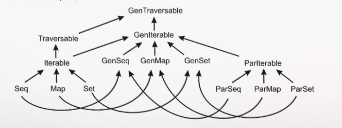
A sequential collection can be converted into a parallel one with .par.
If you’re running in parallel remember avoiding using mutation without proper synchronization.
You can often add ordering to side-effecting operations to make them parallelizable. Example: adding size sorting to a
intersection operation implemented with filter.
Don’t try to modify a parallel collection if an operation is in progress.
“Exception”: TrieMap, with snapshop method, allows modification by reading from a previous version.
Spliter are the Iterator counterpart for parallel collections.
Builder: abstraction to create new collections. Combiner is its parallel counterpart.
Combiner implementation alternatives:
- Most data structures can be constructed in parallel using two-phase construction.
- Efficient concatenation or union (a preferred way when the resulting data structure allows this).
- Concurrent data structure (different combiners share the same underlying daa structure and rely on synchronization
for
+=).
Week 4 - Implementing Combiners
A Combiner is a Builder with an extra method combine to merge two. This operation must be efficient (for
example, execute in O(log n + log m), being n and m the sizes).
You can’t implement efficient enough combiners for arrays because it requires being continuous in memory, so combining requires copying all elements.
Big Data Analysis with Scala and Spark
Week 1 - Spark Basics
RDDs
RDDs are very similar to Scala sequential/parallel collection, but with the data distributed among nodes.
They’re created by transforming an existing RDD, or with an SparkContext, either reading a file
or calling parallelize on an existing collection.
Transformations vs actions
Transformations return new collections, and are lazy. Actions are eager and compute results. Until an action is evaluated, the transformations are not actually performed.
Memory management
Spark model implies performing as much computations as possible in-memory.
You can call .cache() or .persist() on a RDD to avoid reevaluations. It’s very useful on iterations.
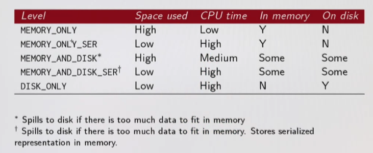
cache uses the default storage level (in memory, regular Java objects). persist allows customization:
- in-memory:
- regular Java objects
- serialized Java objects (more compact)
- on disk
- regular Java objects
- serialized Java objects (more compact)
- both in-memory and on disk (spill over to disk to avoid re-computation)
Topology
Spark is a master/worker topology. The master (the “driver program”) is where the SparkContext is.
Driver program and worker nodes communicate through the Cluster Manager (YARN/Mesos). It manages resources.
Week 2 - Reduction operations & Distributed Key-Value Pairs
Reduction operations
foldLeft/foldRight are not available because they’re not parallelizable. fold is. You often can use aggregate
when foldLeft/foldRight is missed. aggregate is parallelizable and somehow combines both.
Distributed Key-Value Pairs
In Spark, organizing data into key-value pairs are very useful because:
- allow acting on each key in parallel or regrouping data across the network.
- have additional, specialized methods working by key (such as
groupByKey,reduceByKeyorjoin).
Transformations and Actions on Pair RDDs
reduceByKey can be thought as a combination of groupByKey and reduce-ing by key. It’s more efficient than
using it separately because it reduces data transfer among the network.
mapValues is a shorthand of applying a map on a value but still carrying the key around.
Joins
You can do inner, left outer and right outer joins (similar to a relational database).
Week 3 - Partitioning and Shuffling
Shuffling
As you do a groupByKey you get a ShuffledRD, meaning that data must be moved through the network.
Antipattern example: map to project, grouping by key, mapping to get the sizes and sum of the groupings, and collecting.
The grouping moves everything across the network. Alternative 1: map to project, reduceByKey, collect. Alternative 2:
partition by range, reduceByKey.
Partitioning
Partitions never span multiple machines.
The default number of partitions is the number of cores on all executors nodes.
HashPartitioning is the default for grouping by key. Attempts to spread data evenly, based on key
(p = k.hashCode() % numPartitions).
RangePartitioning can be more efficient where the keys can have an ordering defined. It requires the desired number of partitions and a Pair RDD with ordered keys (it’s sampled to create the ranges). RangePartitioning is the default if you sort by key.
If the keys and default partitioning don’t lead to a balanced partitioning you should configure the partitioning.
After setting a partitioning with partitionBy you probably want to persist().
Only groupByKey and sortByKey apply a partitioning. Other transformations preserve the partitioner.
Keep in mind that map loses partitioning, so use mapByKey and reduceByKey if possible.
Optimizing with partitioners
Goal: optimizing for data locality.
It’s probably not important if you’re only transversing once, but it’s key if a RDD is reused.
Rule of thumb: a shuffle can occur when the resulting RDD depends on other elements from the same RDD or another RDD.
Looking at the result type (such as ShuffledRDD[366]) can give information about planned shuffling.
Function toDebugString shows the execution plan.
Operations that can cause shuffling: cogroup, groupWith, join, leftOuterJoin, rightOuterJoin, groupByKey,
reduceByKey, combineByKey, distinct, intersection, repartition, coalesce.
Typical scenarios where you can avoid shuffling with partitioning:
reduceByKey: “pre-partition” to avoid the shuffling. All values will be computed locally.join: if RDDs are already partitioned with the same partitioner, only local operations are needed.
Wide vs Narrow dependencies
Computations on RDDs are represented as a lineage graph, a DAG representing the computations. Lineages graph are the key to fault tolerance: RDDs immutability, functional transformations through higher-order functions and a function for computing the RDD based on its parent RDD. In case of failure you can just recover by recomputing.
RDDs is made of partitions of data, dependencies with the RDDs and its partitions that it was derived from, a function for computing the RDD, and metadata about the partitioning and data placement.
RDD dependencies encode when data must be moved across the network.
Transformations can have two kind of dependencies:
- Narrow: each partition of the parent RDD is used by at most one partition of the child RDD.
No shuffling necessary, pipelining is possible. Example: join with co-partitioned inputs, map, filter…
Full list:
map,mapValues,flatMap,filter,mapPartitions,mapPartitionsWithIndex. - Wide: each partition of the parent RDD may be depended on by multiple child partitions. Requires shuffling. Example: groupByKey, reduceByKey, groupWith, join (without previous co-partitioning)… Full list (of those which can cause shuffling): see “Operations that can cause shuffling” in the previous section. Exception: a join can be narrow instead of wide if there’s copartitioning.
There’s a dependencies method on RDDs that provide this information.
Narrow dependency objects: OneToOneDependency, PruneDependency, RangeDependency.
Wide dependency objects: ShuffleDependency.
Week 4 - Structured data: SQL, Dataframes, and Datasets
Spark SQL
Its goal is not only providing a SQL API. Adding structure to data and computations introduces optimization chances. Spark SQL makes this possible.
Spark SQL is built upon Spark.
Backend components:
- Catalyst: query optimizer. It can leverage reordering of operations or not dropping need data.
- Tungsten: serializer. Column-based, off-heap (free from GC overhead). Packs data in memory.
DataFrames API
DataFrame ~= table. RDDs with a known schema. They are untyped! They contain rows with any random schema.
It’s sometimes difficult express a normal Scala class into a DataFrame (unless it can be expressed as a case class or product).
You can create a Dataframe…
- from an RDD, inferring the schema reflectively (with
toDF). - from an RDD, specifying the schema.
- from a supported structured or semistructured file (JSON, CSV, Parquet, JDBC…).
Supported SQL is largely similar to HiveQL.
Pretty much all the Dataframes API is what you’d expect from a SQL/collections mixture.
Useful methods:
drop: removes rows withnullorNaNin all/some columns.fill: replaces occurrences ofnullorNaNin numeric columns with an specified value.replace: replaces specific values.
Datasets API
DataFrames optimizations + typesafety. In fact, type DataFrame = Dataset[Row]. Typed distributed collections.
They are slightly less performant that DataFrames.
Dataset API unifies DataFrame and RDD APIs. Compared with DataFrames, it allows using higher-order functions.
Antipattern: mapGroups does not support partial aggregation, so it requires shuffling all the data. If you’re using
it to perform an aggregation over each key, you’d better use reduce or an
org.apache.spark.sql.expressions#Aggregator.
Datasets require encoders (code that converts data between JVM objects and Spark SQL internal tabular representation).
They allow optimization. Importing spark.implicits._ is often enough. org.apache.spark.sql.Encoders contains
other useful methods.
Summary:
- Given structured/semistructured data…
- Datasets if you want typesafety or need to work with functional APIs and you don’t need the best performance.
- DataFrames if you want the best, automatic, performance.
- Given unstructured data, use RDD.
RDDs also allows fine-tuning and low-level computations management. Also, they’re needed if you have complex data types that cannot be serialized with encoders.
References
- Books
- Learning Spark
- Spark in Action
- High Performance Spark
- Advanced Analytics with Spark
- Mastering Apache Spark 2
Capstone
The final course is a full project that happens to be a tiler :-).