Specialization content
Google Cloud Spanner
1. Internals
References
1. Code repositories

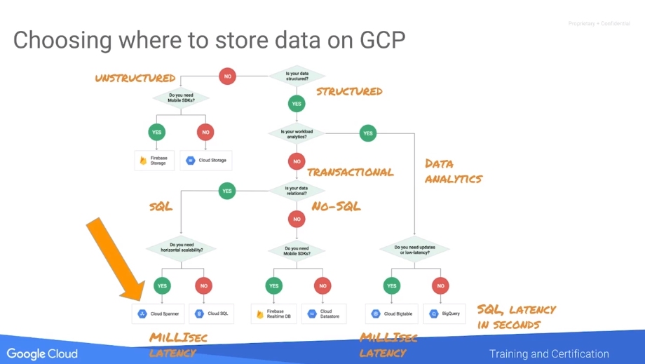
I’m getting closer to Google Cloud solutions, and as some decisions around the platform are not straightforward (such as which database should you use) I took a look at training options and found Data Engineering on Google Cloud Platform Specialization at Coursera. Although it doesn’t get into too much detail, as the platform is huge, it’s a good introduction to the portfolio.

I’ll keep updating the content and references as I learn more stuff:

2019-06: Spanner notes.

Specialization content

The specialization consists of 5 “1 week” (although they can be each completed in a couple of days) courses. I’ve written down some notes, but you can find much more useful documentation at Getting Started.

Google Cloud Platform Big Data and Machine Learning Fundamentals

Using Google Storage as persistent storage for all services make all other services stateless, which is really convenient.

Choosing storage

Choosing storage bis

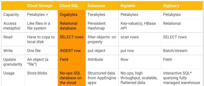
Storage summary:

Cloud Storage: raw files.
Cloud SQL: managed PostgreSQL or MySQL.
Datastore: persistent hashmap. Suitable for hierarchical data. Supports transactions. Useful if you want to be able to filter by properties, which must have an index.
Bigtable: managed HBase, key-value. Useful if you only need filtering by key. Column families group columns that are often queried together. Sweet spot: high throughput, append-only.
BigQuery: warehouse, not real-time.

Some processing services:

Cloud Datalab: managed Jupyter Notebooks.
Pub/Sub: no-ops, serverless global message queue.
TensorFlow: Machine Learning library.
CloudML Engine: managed TensorFlow.

Pre-trained ML models:

Vision.
Speech-to-text.
Natural Language.
Translation.
Video Intelligence.
- Labelling.
- Faces.
- OCR.
- Explicit content.
- Landmarks.
- Logos.

Leveraging Unstructured Data with Cloud Dataproc on Google Cloud Platform

Dataproc: managed Hadoop (Hadoop, Pig, Spark, Hive). Connectors to Bigtable, BigQuery, Cloud Storage.

There are preemptible VMs, cheaper, useful for processing.

Between Google clusters there is high bisection bandwidth, making Google Storage a convenient storage option, instead of using local HDFS units.

Spark uses Resilient Distributed Datasets (RDDs) to abstract data complexity. With Spark you declare a DAG with the transformations, which are lazy, and then run it with actions.

Hadoop/Spark jobs can read from BigQuery, but go through temporary GCS storage.

Serverless Data Analysis with Google BigQuery and Cloud Dataflow

Focus: BigQuery and Cloud Dataflow.

Example arquitecture for data analytics:

Arquitecture for Data Analysis

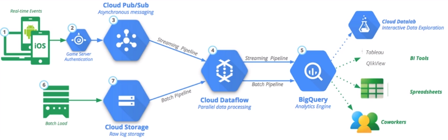
BigQuery

No-ops data warehousing and analytics.

Petabyte-scale querying in seconds.

Standard SQL 2011, including all (?) types and some non-standard ones (STRUCT).

Storing denormalized data has advantages, as the query can be run in parallel more easily. Using nested and repeated columns can bring the best of both worlds.

Querying trigger jobs.

Datasets, which are within projects, contain tables and views (which are queries, live views of a table).

BigQuery uses columnar storage.

User-defined functions limitations:

Only available for the current session (all are temporary).
Can be written in SQL or Javascript.
Can return only <= 5MB.
Each user can run 6 concurrent JS queries per project.
No native code JS functions.

Performance considerations:

Select only the columns that you actually want (remember that BigQuery is columnar storage).
Keep an eye on expensive functions. Example: COUNT vs APPROX_COUNT_DISTINCT.
Do the big joins first (as they will filter data).
Tools:
- Project-level monitoring with Stackdriver.
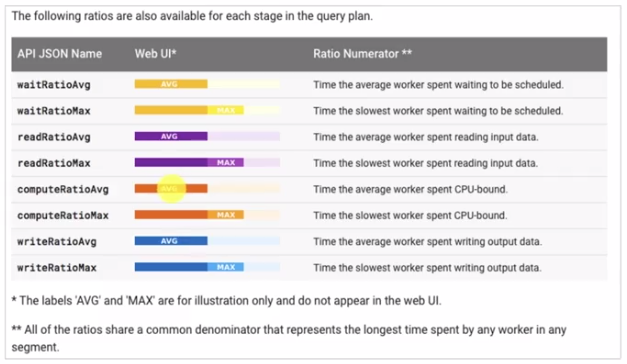
- Explanation plans. Keep an eye on tail skew. In the following example, solid color represents average, pale color means maximum (so you can see that some elements, such as grouping keys with many rows, take much longer).

BigQuery explain plan

BigQuery support “wildcard tables” (select * from project.dataset.table_2016*);

You can also partition tables by timestamp on creation (to avoid the need of partitioning by table name).

Pricing

Pricing is based on the amount of data processed by queries. Reducing queried columns has impact on pricing.

Cloud Dataflow

No-ops data pipelines, both for batch and stream (with the same code).

Runs Apache Beam pipelines (written in Java or Python), which can also be run on top of other runners such as Flink or Spark.

P-collections: parallelizable collections with an apply that generate another PCollection. They’re not bounded (no need to fit in memory, and can even be a stream). By default they’re sharded. You can force disable sharding (for small files, for example) with withoutSharding).

Grouping is similar to MapReduce shuffling.

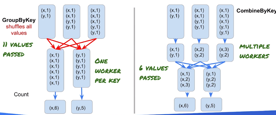
If available, a combine is preferable over a group by key + processing. As a Combiner is commutative and associative, multiple nodes can process the same key before the final aggregation:

Combine vs. group by key + processing

Side inputs

You might need a second data source beyond normal in-memory objects. In those cases you can transform pcollections into “pcollection views” and then pass it as a side input.

Serverless Machine Learning with Tensorflow on Google Cloud Platform

Business Intelligence is about historical data, while Machine Learning is about training the model so it can be applied to unknown data, generating predictive output.

ML comprehends two phases: training a model with lots of data, and inference with the trained model and new data.

Glossary:

Label: true answer.
Input: predictor variable that you can use to predict the label. Input to a neuron.
Example: a label + input.
Feature: input variable used in making predictions. Inputs to the model. There doesn’t have to be a 1 on 1 match from inputs to features. For example, given two inputs x and y, x^2 might be a feature.
Model: math function that takes and input and creates an approximation to a label.
Training: adjust model to minimize error.
Prediction: use a model on unlabeled data.
Regression problem: one where you want to predict a continuous number.
Categorization problem: one where you want to predict one value among a known set of values (categories).
Tensor: n-dimensional array.
Neuron: a way to combine all the inputs into an output.
Hidden layer: layer of neurons with the same sets of inputs.
Hyperparameter: parameter related to the process itself, not feature vales. Example: hidden layer nodes, bucket size of a latlon quantization.
Weights: free parameters that we optimize so that the model contains the data.
Batch size: the amount of data we compute error on.
Epoch: one pass through entire dataset.
Gradient descent: process of reducing error.
Softmax: layer that normalizes a set of output probabilities in order to decide the most likely class in a category decision (example: OCR detection).

Everything that goes into a ML model has to be made numeric, both input and output. For categorization problem the output number is interpreted as a probability.

Adding (hidden) neuron layers adds input combinations.

Datasets should cover all cases, including not only positive cases but also negative ones.

Most common error measurements for optimization:

Regression problems: MSE (Mean Square Error).
Classification problems: cross-entropy. Not intuitive, so after training, in order to decide if the model is good enough, a confusion matrix is used, with the accuracy (successes / total inputs). When the dataset is unbalanced the accuracy is misleading, you can often use precision. Precision is “Positive Predictive Value” (only where the model returned a positive value): positive successes / positive outputs. You can also use recall: positive successes / positive inputs.
- Precision: accuracy when classifier says “yes”.
- Recall: accuracy when the truth is “yes”.

Example: 1000 parking spaces, 990 taken, 10 available. ML identifies only 1. Accuracy: 99.1% (991 / 1000). Precision: 100% (1 / 1). Recall: 10% (1 / 10).

Overfitting: creating a model that fits perfectly to the training dataset but doesn’t generalize to new data (applying it to new data leads to a error very different to the training dataset one).

ML project phases:

Explore.
Create datasets:
- Training data: .
- Validation data: allows picking a final model.
- Test data: once you pick the model, validation data becomes coupled to the model, so you need more new data to test the model with.
Benchmark: set a base heuristic for comparing the model results to.

BigQuery trick: sample data with a hash: MOD(ABS(FARM_FINGERPRINT(CAST(pickup_datetime AS STRING))), 100000) = 1.

TensorFlow

TensorFlow processes numerical computations within a DAG. The nodes represent mathematical operations, and the edges represent arrays (tensors) of data.

It’s not only about ML but about numerical processing.

Exposes high level APIs on top of a C++ core that runs on different hardware (CPU, GPU, TPU…).

The ML API is the estimator API.

Cloud ML Engine is a serverless TensorFlow run engine.

In order to separate the declaration of the DAG from the execution, TensorFlow has a lazy execution model. That way it can, for example, execute nodes remotely or in different hardware. That might require changing the graph.

Effective ML requires big data, feature engineering (creating good features, transforming inputs…) and model architectures.

Feature engineering:

Features must be related to the objective.
Causality: Available at production (prediction) time.
Numeric
Enough examples: 5+ examples for each value.
Categorical values must be one-hot encoded.
Feature crosses: add human insight to make relationship between features explicit.
Bucketize real values into bins and use it as a categorical feature.
Sparse (categorical, “wide”) features typically work well with linear models. Dense (numerical) features, with deep models. If there are both, we can use deep models and connect directly inputs with outputs for sparse features. This is called “wide-and-deep network”.

Cloud AutoML automates the creation of a model.

Building Resilient Streaming Systems on Google Cloud Platform

Streaming => processing of unbounded datasets.

Challenges:

Variable volumes require scaling in a fault-tolerant manner (with Pub/Sub).
Latency will happen, it requires processing (with Dataflow) of late/error data.
Real-time insights (with BigQuery or Bigtable) are the desired output.

Pub/Sub

Serverless message bus.

Messages persist for 7 days.

Works with topics and subscriptions. Subscribers register at subscriptions. Each subscription supports multiple subscribers. Subscribers of the same subscriptions can have different paces. Subscriptions collect several topics as well.

At least once delivery guarantee. Order and unicity is not guaranteed.

Dataflow handles deduplication and order if needed.

Fan-in: multiple subscribers listening to the same topic.

Fan-out: multiple publishers publishing to the same topic.

Pull & push delivery flows.

In push deliveries, Pub/Sub initiates the communication to the subscribers. It requires https (it must be a server application) for webhooks.

In pull deliveries, the subscriber has to poll for new messages. Subscriber receives a ack id and it must send a ACK so Pub/Sub knows that the message was successfully delivered and can delete it.

You can pass metadata (key-value pairs) with the messages. Sending the timestamp of the message is often very useful.

Messages can be sent in batches, reducing the network cost.

Dataflow & streaming

Apache Beam is an unified model for batch and stream (to avoid needing two pipelines). Can run on multiple runtimes.

Introduces windowing: shuffles events in time windows based on the event timestamp (when the event occur).

Types of windows:

Fixed.
Sliding.
Sessions.

Allows combining batch, micro batch and stream.

Setting id label at Dataflow when you read from Pub/Sub adds only-once semantics (as long as a valid id is set on publish).

Late data

Remember: event time != processing time.

The default setting triggers new computations if data is arrived late.

Dataflow learns from the skew of the messages over time and computes an heuristic about if a window is likely to be closed or not. The “watermark” is that heuristic about the progress. Based on this, Dataflow chooses when to emit the event of window closed.

Elements added: how many elements exited a given step.

Data watermark age: the age (time since event timestamp) of the most recent item of data that has been fully processed by the pipeline.

System lag: the current maximum duration that an item of data has been awaiting processing, in seconds.

What results are calculated: transformations Where in event time are results calculated: event-time windowing When in processing time are results materialized: watermarks, triggers, and allowed lateness. How do refinements of results relate: answered via Accumulation modes.

BigQuery & streaming

BigQuery supports streaming ingest, data is available in seconds.

Cloud Spanner

Higher throughput and lower latency than BigTable.

Transactional, horizontally scalable (for use cases where Cloud SQL, backed by MySQL or PostgreSQL, is not enough).

BigTable

Key/value store. Key determines the tablet where the data is going to be stored (and you want it to be evenly distributed).

Higher throughput and lower latency than BigTable.

For data analytics.

More expensive than BigQuery.

Separates computing and storage. Bigtable clusters contain not data but metadata, pointers to Colossus (Google filesystem).

HBase API.

In order to add data you create mutations.

Schema design

Docs.

Two types of designs:

For dense data (where all columns have values) you can create a normal table. Example: for user information, you’d have the username as key, with one user_information family with the columns (name, gender…).
For sparse data (such as relationships) you can set up keys with the relation information. For example, for a “following” relationship, you can have a key that is the concatenation of the hashes of the follower and the following users, and one column with the followed username.

Cloud Bigtable tables are sparse. Empty columns don’t take up any space. As a result, it often makes sense to create a very large number of columns, even if most columns are empty in most rows. In addition, it often makes sense to treat column qualifiers as data.

That said, you should avoid splitting your data across more column qualifiers than necessary, which can result in rows that have a very large number of non-empty cells. It takes time for Cloud Bigtable to process each cell in a row. Also, each cell adds some overhead to the amount of data that’s stored in your table and sent over the network. For example, if you’re storing 1 KB (1,024 bytes) of data, it’s much more space-efficient to store that data in a single cell, rather than spreading the data across 1,024 cells that each contain 1 byte. If you normally read or write a few related values all at once, consider storing all of those values together in one cell, using a format that makes it easy to extract the individual values later (such as the protocol buffer binary format).

Choosing a key

Queries are efficient if they use the row key, prefix or range. Corollary: the most common query determines the key.

Rows are stored in ascending order of the key (that’s why if you often query the most recent events you should use a inverse timestamp at the key), and only one key can be indexed.

If you often want to retrieve the most recent records, you should use a reverse timestamp so the most recent records are the most recent.

You want to distribute evenly across rows (keys). Avoid these keys to avoid hotspotting:

Domains: not all domains are equally active.
Sequential user IDs: newer users are more active.
Static identifiers: frequent used identifiers overload a single tablet.

Families

Related columns should be grouped in the same family. Change rate at columns within a same family should be similar (columns that often get changed together).

You can use up to about 100 column families while maintaining excellent performance.

The names of your column families should be short, because they’re included in the data that is transferred for each request.

Performance

General considerations:

Bigtable learns to configure itself. Looks at access patterns and reconfigures itself. For example, it moves metadata across nodes if some are overused. So, don’t try doing load tests on the first minutes.
It also redistributes storage (updating pointers).
It should support ~ 10kQPS @ 6 ms latency on SSD (220 MB/s) both for reads and writes.
It should support ~ 10kQPS @ 50 ms latency on HDD (180 MB/s) for reads, and ~500 QPS @ 200 ms for writes.
Performance scales linearly with the number of nodes.
Design the schema so the reads and writes can be distributed evenly.
Increasing the amount of data per row reduces the number of rows per seconds.
Increasing the amount of cells per row reduces the number of rows per seconds.
In general, keep all information for an entity in a single row. An entity that doesn’t need atomic updates and reads can be split across multiple rows. Splitting across multiple rows is recommended if the entity data is large (hundreds of MB)

Google Cloud Spanner

Spanner is not part of the certification, but here are some notes about what I’m learning about it.

TL;DR: relational, transactional, horizontally scalable database.

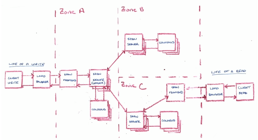
Internals

It uses TrueTime, a system based on atomic clocks that provide not only a very accurate moment in time but also bounded (predictable) clock uncertainty. Timespan is used to create the global ordering of the events. Spanner assigns globally meaningful commit timestamps to transactions, even for distributed ones. Those timestamps reflect serialization order. Serialization order satisfies external consistency (linearizability).

Lifespan of a request (read/write)

It uses Paxos as the consensus protocol to pick the leader.

One design goal is serving data (almost) always from local storage. If the replica doesn’t have it, it waits until Paxos propagate it.